반응형
- 의류 이미지 분류 (패션 MNIST)

- 의류 데이터 준비
※ 텐서플로 최신 버전 설치
!pip install tensorflow_gpu==2.6.0
1. 텐서플로 임포트
import tensorflow as tf
2. 텐서플로 버전 확인
tf.__version__


##출력: '2.6.0'
3. 패션 MNIST 데이터 세트 불러오기
(x_train_all, y_train_all), (x_test, y_test) = tf.keras.datasets.fashion_mnist.load_data()
4. 훈련 세트의 크기 확인
print(x_train_all.shape, y_train_all.shape)


##출력: (60000, 28, 28) (60000,)

5. imshow() 함수로 샘플 이미지 확인
import matplotlib.pyplot as plt

plt.imshow(x_train_all[0], cmap='gray')
plt.show()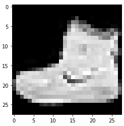
6. 타킷의 내용과 의미 확인
print(y_train_all[:10])


##출력: [9 0 0 3 0 2 7 2 5 5]
7. 타깃 분포 확인
class_names = ['티셔츠/윗도리', '바지', '스웨터', '드레스', '코트', '샌들', '셔츠', '스니커즈', '가방', '앵클부츠']

print(class_names[y_train_all[0]])


##출력 : 앵클부츠
8. 훈련 세트와 검증 세트 고르게 나누기
from sklearn.model_selection import train_test_split

x_train, x_val, y_train, y_val = train_test_split(x_train_all, y_train_all, stratify=y_train_all, test_size=0.2, random_state=42)
9. 입력 데이터 정규화
x_train = x_train / 255
x_val = x_val / 255
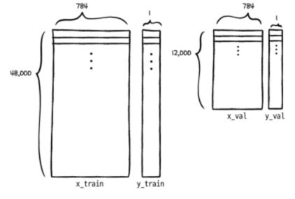
10. 훈련 세트와 검증 세트 차원 변경
x_train = x_train.reshape(-1, 784)
x_val = x_val.reshape(-1, 784)

print(x_train.shape, x_val.shape)


##출력: (48000, 784) (12000, 784)
반응형
- 타깃 데이터를 준비하고 다중 분류 신경망 훈련
1. 타깃을 원-핫 인코딩으로 변환
from sklearn.preprocessing import LabelBinarizer
lb = LabelBinarizer()
lb.fit_transform([0, 1, 3, 1])


##출력:
array([[1, 0, 0],
       [0, 1, 0],
       [0, 0, 1],
       [0, 1, 0]])
2. 배열을 각 원소를 뉴런의 출력값과 비교
tf.keras.utils.to_categorical([0, 1, 3])


##출력:
array([[1., 0., 0., 0.],
       [0., 1., 0., 0.],
       [0., 0., 0., 1.]], dtype=float32)

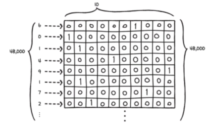
3. to_categorical 함수 사용해서 원-핫 인코딩
y_train_encoded = tf.keras.utils.to_categorical(y_train)
y_val_encoded = tf.keras.utils.to_categorical(y_val)

print(y_train_encoded.shape, y_val_encoded.shape)


##출력: (48000, 10) (12000, 10)

print(y_train[0], y_train_encoded[0])


##출력: 6 [0. 0. 0. 0. 0. 0. 1. 0. 0. 0.]
4. MultiClassNetwork 클래스로 다중 분류 신경망 훈련
fc = MultiClassNetwork(units=100, batch_size=256)
fc.fit(x_train, y_train_encoded, x_val=x_val, y_val=y_val_encoded, epochs=40)
5. 훈련 손실, 검증 손실 그래프와 훈련 모델 점수 확인
plt.plot(fc.losses)
plt.plot(fc.val_losses)
plt.ylabel('loss')
plt.xlabel('iteration')
plt.legend(['train_loss', 'val_loss'])
plt.show()
fc.score(x_val, y_val_encoded)

##출력: 0.8150833333333334


np.random.permutation(np.arange(12000)%10)

##출력: array([4, 6, 3, ..., 0, 6, 6])


np.sum(y_val == np.random.permutation(np.arange(12000)%10)) / 12000

##출력: 0.10325
※ 해당 내용은 <Do it! 딥러닝 입문>의 내용을 토대로 학습하며 정리한 내용입니다.
반응형
'딥러닝 학습' 카테고리의 다른 글
| 8장 이미지 분류 - 합성곱 신경망 (1) (0) | 2023.03.16 |
|---|---|
| 7장 여러개를 분류 - 다중 분류 (3) (0) | 2023.03.15 |
| 7장 여러개를 분류 - 다중 분류 (1) (0) | 2023.03.13 |
| 6장 2개의 층을 연결 - 다층 신경망 (4) (0) | 2023.03.12 |
| 6장 2개의 층을 연결 - 다층 신경망 (3) (0) | 2023.03.11 |


